WHAT ARE THE COMBASE BROTH MODELS?
ComBase broth models predict the response of a range
of pathogens and spoilage microorganisms to key factors (temperature, pH and
salt concentration, etc) characterising the food environment. The majority of
its models predict the growth/survival of foodborne pathogens as a function of
temperature, pH and salt concentration, but in some cases the effect of an
additional fourth environmental factor, such as the concentration of carbon
dioxide or organic acids is modelled, too. The models can simultaneously
produce predictions for up to four microorganisms. They are also capable of
predicting the bacterial response to dynamic temperature environments. This is
especially useful when the changes in the storage temperature are known, for
example, from a temperature logger. In this case, the data from the temperature
logger (up to a hundred time-temperature points) can be entered into an input
box.
WHY THEY MIGHT BE USEFUL TO ME?
If your interests include food safety, then the predictive microbiology
capability provided by this user friendly, web based tool will be useful to you.
It will enable you to judge more easily the effect of production and storage
regimes and changing product formulations on the possible growth of pathogens or
spoilage organisms.
WHO IS USING THE COMBASE BROTH MODELS?
They are expected to be used by a large range of people including
quality assurance, product development and legal professionals, legislators,
retailers, trainers and students. Benefits may include a reduction in the amount
of microbiological testing that is necessary for a product. However, please note
that the use of ComBase broth models is not a substitute for testing products
before release.
WHAT IS THE MODELLING BACKGROUND OF THE COMBASE BROTH MODELS?
ComBase broth models are based only on output from laboratory
experiments observed in culture media under well controlled laboratory
conditions. Variation of cell concentration is described by a mathematical
(growth or survival) curve and this is called a primary model. Secondary models
describe how the parameters of primary models depend on environmental factors
such as temperature, pH and water activity. These are described by mathematical
functions, and, by interpolation, the cell concentration against time can be
predicted for any combination of conditions.
Baranyi and Roberts (1994) model is used as the primary model. To create the secondary models,
the logarithms of the specific growth rates were described as a function of the
(possibly rescaled) environmental factors by a standard quadratic multivariate
polynomial. Standard second order
polynomials model the effect of temperature, pH, and Aw values on the logarithm
of the growth rate. The maximum specific growth rate is the main model parameter
for ComBase broth models. The other key parameter (in place of lag) is the ‘initial
physiological state’ (phys. state). The phys. state value is a dimensionless
number between 0 and 1; if phys. state = 0, then there is no growth and the lag
time is infinite; if phys. state=1, there is no lag and growth will commence
immediately. It has a similar role to the inoculum size but is an initial
parameter quantifying the history of the cells. The value for this parameter can
be selected by the user but because the user is rarely able to provide its true
value, the user can set it to a value typical for the experiments used to develop the model. It is advised that
users try different values for the physiological state, to study its effect on
the growth curve. For further information regarding this ‘initial physiological
state’ parameter, see Baranyi and Roberts (1994).
REFERENCES
Baranyi, J. and Roberts, T.A (1994). A dynamic approach to predicting bacterial
growth in food. International Journal of Food Microbiology 23, 277-294.
Gibson A. M., Baranyi J., Pitt I., Eyles M. J. and Roberts (1994). Predicting fungal
growth: the effect of water activity on four species of Aspergillus. International Journal of Food Microbiology 23, 419-431.
Resnik, S. L. and Chirife, J. (1988). Proposed theoretical aw values at various temperatures for
selected solutions to be used as reference sources in the range of microbial
growth. Journal of Food Protection 51, 419-423.
ComBase broth models can be used to make predictions in
either a static temperature or under fluctuating (changing) temperature
conditions. They can provide up to four simultaneous predictions and include growth and survival curves
as well as thermal and non-thermal death curves
1.- GENERATING A SINGLE PREDICTION AT STATIC
TEMPERATURE
Select the model category: select
'growth model' for prediction of bacterial growth or 'thermal death model' for
prediction of thermal inactivation.
Select the required model: The first step in producing a
prediction is to select a model. A drop-down menu of models can be viewed in the ‘select a model’ listbox.
Click on the arrow to
view the full list. The model required for the organism of interest can then be
highlighted and selected from the menu. Many of the models encompass three
environmental factors (temperature, pH and water activity). Some models also
have an additional fourth environmental factor e.g. CO2 or lactic
acid. One basic principle of empirical modelling is that one should not
extrapolate: predictions should not be made outside the region of observations.
The limits of the selected model for each environmental factor appear below the
input fields.
Input environmental factor values: Default values for the
environmental factors (temperature, pH, water activity, etc) automatically
appear in each of the input fields. Default values should be replaced by values
of interest to you. The range within which input values must fall is indicated
beside the input field for each of the factors. If values outside the range are
selected, an error message will be generated. Water activity can be expressed in
terms of sodium chloride (%NaCl) or water activity. Water activity can be
calculated from NaCl concentration by toggling between NaCl and Aw buttons (it
is assumed that the salt is dissolved in water). The %NaCl values are
transformed into water activity values by the formula:
Aw=1-%NaCl*(5.2471+0.12206*%NaCl)/1000 (Resnik and Chirife,
1988)
To get a prediction:When a four-factor model has been selected, values are also
required for the 'Factor 4' field. The default value for
the initial count is log10cell concentration = 3 (i.e. 103
cells/ml). For the physiological state, the default value is the value which was
typical for the curves providing the base for the models. It is not possible to
select ‘initial level’ values for thermal death models as results are provided
as a relative decrease in log concentration.
The prediction output: The right-hand output panel now shows
a graphical representation of the prediction. A statement of maximum growth rate
and doubling time (or maximum death rate and D-value) are presented below the
graph. Additionally, each of the time vs. cell concentration data points for the
prediction are listed below the graph and may be selected and copied for use in
other applications (e.g. Excel).
2.- GENERATING MULTIPLE PREDICTIONS AT STATIC TEMPERATURE
Multiple
predictions are generated in a similar manner to single predictions. Click the
'add prediction' button up to three times to create multiple input sections. A total
of four simultaneous predictions can be made. Using this feature, it is possible
to compare the responses of a number of different organisms to a single set of
environmental conditions or for a single microorganism to varied environmental
conditions. To return to a single prediction, click the 'remove last row' button
the required number of times.
3.- GENERATING A SINGLE PREDICTION UNDER FLUCTUATING
TEMPERATURE
The tool does not only allows prediction to be
made for static temperature conditions but also predictions under certain
fluctuating (changing) temperature conditions. For example, predictions could be
made from data representing the fluctuating time vs. temperature profile
expected or measured for the following processes in sequence: the later stages
of cooling, storage within the factory, storage during transportation, storage
at retail premises, possible purchaser temperature abuse followed by domestic
storage for the organisms Listeria monocytogenes and non-proteolytic
Clostridium botulinum using the appropriate growth models. This
'fluctuating temperature' feature may also be useful to demonstrate the affect
of a thermal process using logged data which falls within the relevant
temperature range of the thermal death model.
Select Dynamic prediction:Input the temperature profile in the Time/Temperature table. For details about how to input your
temperature profile, refer to the Data Input section
Select the required model:
Select the required model as described for static temperature predictions.
Input environmental factor values:
Values for environmental factors for ‘changing temperature’
predictions should be entered as described for ‘static temperature’ predictions
except for the values pertaining to temperature.
The prediction output: The
right-hand output panel now shows time vs. cell concentration data for the given
prediction (white) alongside the selected time vs. temperature profile (green).
No statements of maximum growth rate or doubling time are provided as these
fluctuate according to the time vs. temperature input. However, each of the time
v. cell concentration data points for the prediction are listed on the "Data Points" tab
and may be selected and copied for use in other applications.
GENERATING MULTIPLE PREDICTIONS AT FLUCTUATING TEMPERATURE
This process is performed in a similar manner to
that already described. This facility can be used to compare organisms or key
parameters for a single fluctuating temperature profile. It is not possible to
make predictions when the temperature ranges of the models do not overlap.
REFERENCES
Resnik, S. L. and Chirife, J. (1988). Proposed
theoretical aw values at various temperatures for selected solutions to be used
as reference sources in the range of microbial growth. Journal of Food
Protection 51, 419-423.
For further information, read the user manual
1. What is the Phys. state value?
The Phys. state (or “initial physiological state”) is a dimensionless number between 0 and 1 expressing the physical suitability of the cells to their environment. If its value is 0, then growth will not occur (infinite lag); if the value is 1, then growth will commence immediately, without lag.
The duration of the lag depends not only on the actual environment (temperature, pH water activity, etc) but also on the history of the cells. Stresses (e.g. thermal, osmotic, acid) can significantly increase the lag times. An example of this history dependence of the lag duration is given in the chart below. Listeria monocytogenes was grown in the same medium at 15°C after sub-cultures from different conditions. The growth rate is similar in both cases but significant differences in lag durations are observed.
The phys. state value quantifies the effect of the history on the bacterial lag time. The lag time can be derived from the phys. state value using the formula:
lag = -log(Phys. state)/Max.rate
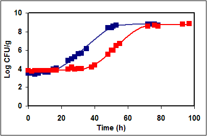
Figure 1. Growth of Listeria monocytogenes in broth, at 15°C after different subculturing procedures.
2. Which value should I input for the Phys. state value?
The default physiological state is set to 1, meaning already adapted cells, i.e. no lag time. Because the user is rarely able to provide its value, the user can set it to a value typical for the experiments used to develop the model. The user might experimentally evaluate the phys. state value suitable for the pre-incubation conditions of interest. This can be done by fitting growth curves obtained after incubatory conditions simulating the history of the cells (e.g. stress). Once the lag and the growth rate are calculated, the Phys. state can be deduced by the equation:
Phys. state= 10^(-lag x Max.rate)
It is suggested that users try different values for the physiological state, to study its effect on the growth curve.
1. Format requirements:
The time/ temperature should be inserted in the texbox on the 'changing temperature' page in the format illustrated and described below:
| 0 |
12.5 |
| 10 |
12.5 |
| 10.5 |
18.4 |
| 14 |
20 |
| 15 |
8 |
| 25 |
8 |
| 26 |
12 |
| 30 |
15 |
For each time temperature record of your profile, time is to be entered first (in hours) then temperature (in °C).
You must use the 'point' symbol "." as the decimal separator.
The profile can be typed directly or may be copied from another application (e.g. Excel spreadsheet, text file) and pasted.
2. Modelling requirements:
All temperature values must be within the range for the models selected.
There must be a minimum of 4 and a maximum of 100 (time vs. temperature) records in your profile.
The records must be recorded in chronological order.
The first time-point must be '0'.
The last time point must be less than or equal to '5000' hours.
Revised Models
Until recently, the first version of the ComBase Predictor had a problem with the broth four-factor growth models: under certain combinations of conditions (like high CO₂ or added preservatives), it might have shown bacteria growing faster than under less stringent environmental conditions —when in fact, they shouldn't.
This happened only under conditions around which there were no measured data (extrapolations).
Thanks to feedback from users, these problems were identified.
The ComBase Predictor update (v1.1), corrects this by applying a stricter mathematical “clean-up”, called backward elimination, of non-significant terms in the formulae. This ensures that predictions now follow a more biologically sound and expected (from experience) pattern.
While the first version, ComBase Predictor v1.0 served its purpose well, ongoing research and user feedback have pointed to directions for further developments. This is natural in predictive sciences, much like in weather forecasting: models evolve as we learn more and refine the methods. The updated version, ComBase Predictor v1.1, brings a more reliable mathematical treatment of the data, especially when multiple environmental factors are involved. Users can expect further improvements within a year or two as development and refinement continues.
Summary of Revisions
For complete details, refer to the following PDF: ComBase Predictor Update December 2025.